PhysDNet: Physics-Driven Gradient Amplification for Real-Time Image Dehazing

NeurIPS 2026

Rayen Dhahri¹ Lei Sun² Victor Javier Kartsch Morinigo³ Alice Pagnoux³ Luca Benini^3,4 Danda Pani Paudel² Luc Van Gool²

¹Independent Researcher ²INSAIT, Sofia University “St. Kliment Ohridski” ³ETH Zurich ⁴DEI, University of Bologna

Contact: rayendhahri@gmail.com

Overview illustration: a smoke-filled corridor and simulated sparse LiDAR enter PhysDNet; differentiating through the physics inversion amplifies gradients in low-transmission regions during training; the restored image reveals a person and an obstacle for detection — **Overview.** Hazy imagery and sparse LiDAR are fused by PhysDNet. During training, differentiating through the physics inversion scales gradients by (t̂+ε)⁻², focusing learning on low-transmission regions at zero inference cost. Conceptual illustration of a potential emergency-response application; the scene and LiDAR are schematic, not experimental results.

Abstract

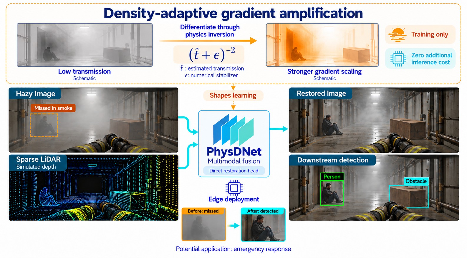
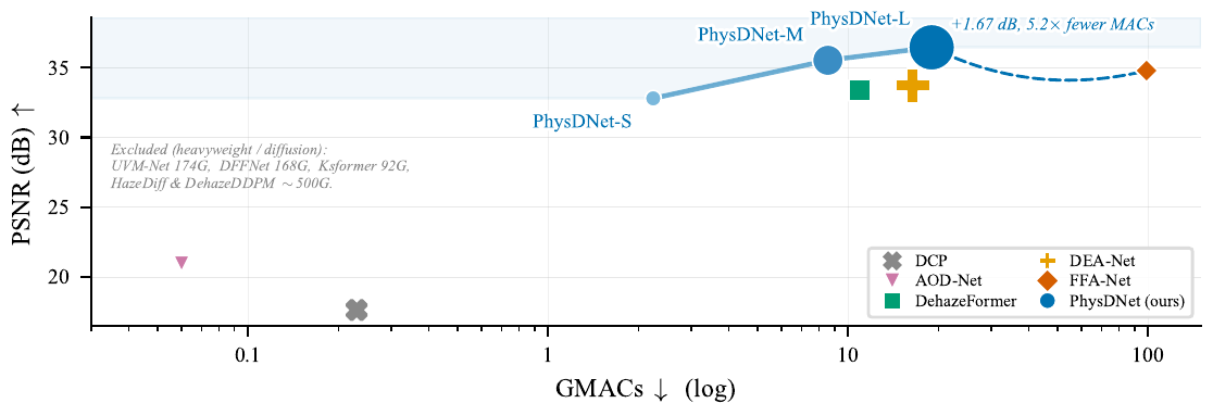
Modern dehazing networks are often computationally expensive and overfit to synthetic haze, limiting real-time deployment. This underscores an urgent demand for efficient, high-fidelity restoration methods that can operate on resource-constrained edge devices in practical, dynamic environments. We introduce PhysDNet, a lightweight multimodal architecture that fuses NIR imagery with sparse LiDAR depth and is trained with a physics-constrained dual-head objective. Differentiating through a fixed Koschmieder inversion induces density-adaptive gradient amplification, acting as an implicit resource allocation mechanism that concentrates learning on heavily degraded regions without increasing inference cost. PhysDNet delivers superior restoration with minimal capacity and enhanced training efficiency, facilitating real-time deployment on edge devices without increasing inference overhead. On the Seeing Through Fog benchmark, PhysDNet outperforms competitors by 1.67 dB at 5.2× lower compute and recovering 54.9% of fog-induced detection loss. Ablations and cross-domain evaluations show that physics-guided training improves generalization including under non-homogeneous haze that violates the Koschmieder assumption. PhysDNet further demonstrates compatibility with fixed-function NPUs, running at 29/45/99 FPS at <4 W across L/M/S variants.

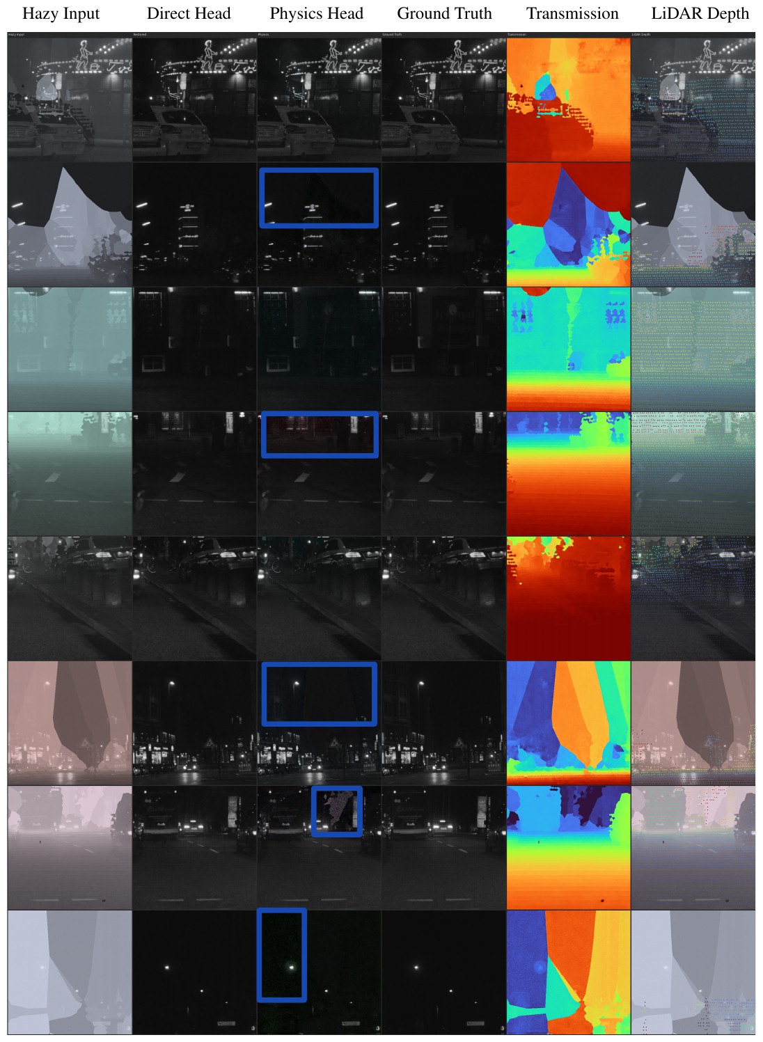
Real STF Example

Foggy NIR-gated frame of a snowy street at night

Hazy NIR inputPhysDNet

Drag across the image to compare a hazy gated-NIR frame from Seeing Through Fog with PhysDNet's restoration. PhysDNet also receives the sparse projected LiDAR depth shown by the toggle.

Overlay sparse LiDAR returns

36.46 dB PSNR on STF, +1.67 dB over FFA-Net at 5.2× lower compute
54.9% of fog-induced YOLOv8 detection loss recovered
29 / 45 / 99 FPS (L / M / S) on a fixed-function NPU at <4 W, INT8
Physics head is used only in training: zero inference overhead

Method

PhysDNet architecture diagram — **Figure 1. PhysDNet architecture.** Dual encoders extract NIR and sparse-depth features, merged by mask-aware gating with Squeeze-and-Excitation at the bottleneck. The shared representation feeds a direct head (deployed at inference) and a physics head (training only). Backpropagating through the Koschmieder inversion scales gradients by (t̂+ε)⁻², concentrating optimization on heavily degraded regions at zero inference cost.

Interactive · architecture explorer

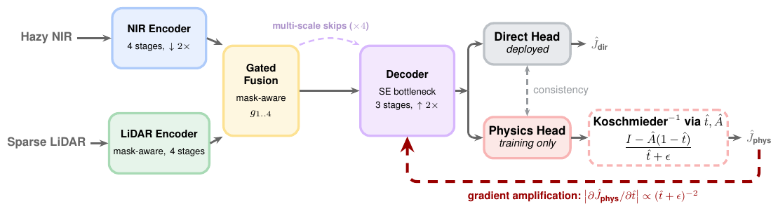
Click any block for its role, tensor shape (PhysDNet-M, base width c = 64; S/M/L use c ∈ {32, 64, 96}) and equation.

Density-adaptive gradient amplification

The physics head predicts transmission t̂ ∈ [0.05, 0.95] and a global airlight Â, then inverts the scattering model I = J·t + A(1 − t) in closed form: Ĵ_phys = (I − Â(1 − t̂)) / (t̂ + ε). This inversion has no learnable parameters. Its derivative, ∂Ĵ_phys/∂t̂ = (Â − I) / (t̂ + ε)², scales the gradient reaching the shared encoder by up to ≈400× in dense fog relative to clear air. The result is an implicit hard-example mining along the transmission axis, with no extra hyperparameters and no inference cost.

Bar charts of gradient magnitude versus transmission for PhysDNet-M and NoPhy — **Figure 3. Density-adaptive gradient amplification.** PhysDNet-M follows the (t+ε)⁻² scaling and concentrates gradients on low-transmission regions (up to ~694× the NoPhy baseline), unlike the flat NoPhy profile.

Hazy input, predicted transmission, gradient magnitude map and physics output on a real fog frame — **Figure 6. Empirical gradient map on a real STF fog frame.** Hazy input, predicted t̂, analytical gradient magnitude |∂Ĵ_phys/∂t̂|, and physics-restored output. High-gradient regions align spatially with low-transmission regions.

Interactive · Koschmieder model and its inversion

scattering coefficient β 0.040

airlight A 0.80

error in t̂, δ +0.020

clear scene J

transmission t = e^−βd

hazy I = J·t + A(1−t)

inversion with t̂ = t + δ

mean t – inversion error, near field – inversion error, far field – far / near –

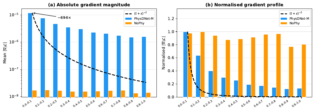
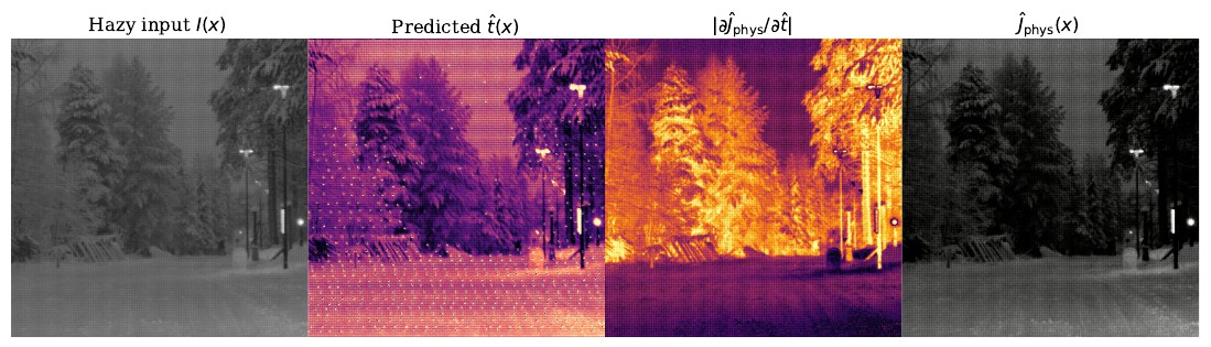
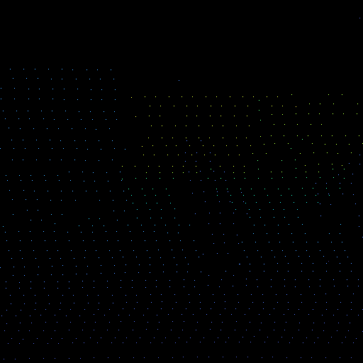
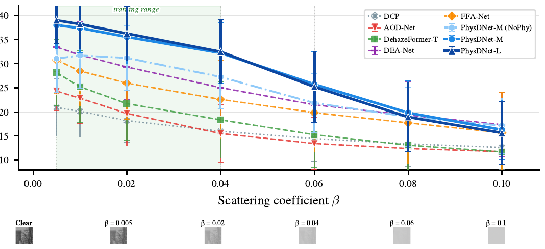
A fixed error δ in t̂ produces a restoration error δ(A − J)/(t + δ): harmless where t is high, amplified where fog is dense. This t-dependence is why the gradient through the inversion concentrates on dense haze. β covers the paper's 0.005–0.10 sweep. For illustration, J is PhysDNet's restored frame and d is a dense depth map interpolated from this frame's own sparse LiDAR returns (about 4–72 m). Near field: d < 15 m; far field: d > 40 m.

Results

Restoration quality on Seeing Through Fog

**Table 1.** STF validation set (1,299 frames), direct head. PhysDNet-M: mean ± SE over 3 seeds. Best in bold, second underlined.
Method	Input	Res.	Params (M)	GMACs	PSNR (dB) ↑	SSIM ↑
DCP	NIR	256	0	—	17.62	0.5992
AOD-Net	LiDAR+Gated	256	0.002	0.06	20.95	0.7329
DehazeFormer-T	NIR	512	1.36	10.92	33.38	0.9348
FFA-Net	NIR	512	0.77	98.57	33.90	0.9474
FFA-Net	NIR+LiDAR	512	0.77	98.73	34.79	0.9516
DEA-Net	NIR	256	3.65	16.42	33.71	0.9588
DEA-Net	LiDAR	256	3.65	16.44	33.53	0.9572
PhysDNet-S	NIR+LiDAR	256	0.72	2.24	32.80	0.9331
PhysDNet-M	NIR+LiDAR	256	2.95	8.56	35.55±0.07	0.9566±0.0009
PhysDNet-L	NIR+LiDAR	256	6.59	18.98	36.46	0.9606

Best-resolution row per baseline shown; the paper's Table 1 lists every resolution and input combination.

PSNR versus GMACs scatter plot — **Figure 2. Accuracy vs. computational cost on STF.** PhysDNet establishes a new Pareto front in the edge-deployable region. PhysDNet-L outperforms FFA-Net by +1.67 dB at 5.2× lower compute; PhysDNet-S retains competitive accuracy at ultra-low compute.

Physics head ablation

**Table 2.** Removing the physics head (NoPhy) from an identical ch64 model.
Variant	Physics head	Params (M)	PSNR (dB)	SSIM	mAP (%)	ΔmAP
PhysDNet-M	✓	2.95	35.55	0.9569	11.70	+3.05
PhysDNet-M NoPhy	×	2.91	30.02	0.9263	10.70	+2.06
Difference		−0.04	−5.51	−0.0306	−1.00	−0.99

Grid of hazy inputs, direct head, physics head, ground truth, transmission and LiDAR depth for eight scenes — **Figure 11. Dual-head outputs on synthetic STF fog.** Blue boxes mark dense-haze regions where the physics head shows noise amplification; the direct head suppresses these artifacts by relaxing the rigid physical assumptions.

Downstream object detection

**Table 3.** YOLOv8-M on 426 STF val frames with synthetic fog (β = 0.06). Recovery = ΔmAP / |fog degradation|.
Condition	AP_veh	AP_pers	AP_cyc	mAP (%)	ΔmAP	Recovery
Clean (upper bound)	33.95	7.97	1.05	14.33	—	—
Foggy (β = 0.06)	18.09	5.42	2.42	8.64	−5.68	—
AOD-Net (NIR)	15.14	4.66	1.27	7.02	−1.62	—
DehazeFormer-T (NIR)	16.37	5.74	1.65	7.92	−0.72	—
FFA-Net (NIR)	24.37	6.30	1.32	10.66	+2.02	35.6%
DEA-Net (NIR)	25.82	5.82	1.66	11.10	+2.45	43.1%
PhysDNet-S	24.49	5.94	1.22	10.55	+1.91	33.6%
PhysDNet-M	27.65	6.45	0.99	11.70	+3.05	53.7%
PhysDNet-L	27.60	6.70	0.99	11.76	+3.12	54.9%

Detections on foggy image, FFA-Net output, PhysDNet-M output and clean image — **Figure 4. Downstream detection after dehazing (β = 0.06).** PhysDNet-M recovers scene contrast and enables more accurate detections than FFA-Net. Dashed white: ground truth; solid coloured: predictions.

Out-of-distribution fog density

PSNR versus scattering coefficient beta for all methods — **Figure 12. PSNR vs. fog density β** (256×256, A = 0.8; green band is the training range). PhysDNet-M keeps the highest PSNR at every density, with a >6 dB margin over the best baseline at β = 0.06, and degrades gracefully outside the training distribution.

Zero-shot cross-domain generalization

Trained on STF only and evaluated on O-HAZE and I-HAZE with no LiDAR at test time (NIR→RGB, synthetic→real, outdoor→indoor). PhysDNet-M improves PSNR-Y over DEA-Net by +0.53 dB on O-HAZE and +0.62 dB on I-HAZE; on non-homogeneous NH-HAZE, which violates the Koschmieder assumption, it still leads by +0.15 dB, and removing the physics head costs 0.54 dB.

**Table 4.** Zero-shot results (luminance and RGB metrics).
	O-HAZE (outdoor)				I-HAZE (indoor)
Method	PSNR-Y	SSIM-Y	PSNR-RGB	SSIM-RGB	PSNR-Y	SSIM-Y	PSNR-RGB	SSIM-RGB
AOD-Net	15.11	0.5000	14.88	0.4931	14.69	0.5824	14.51	0.5724
FFA-Net	19.20	0.7177	18.49	0.6968	15.82	0.6521	15.48	0.6402
DehazeFormer-T	19.48	0.6839	18.81	0.6641	15.86	0.6142	15.56	0.6050
DEA-Net	19.92	0.7042	19.20	0.6854	16.31	0.6455	16.02	0.6362
PhysDNet-S	19.89	0.7190	19.21	0.6989	16.81	0.6895	16.49	0.6734
PhysDNet-M	20.45	0.7461	19.65	0.7253	16.93	0.6947	16.59	0.6795
PhysDNet-M (NoPhy)	18.92	0.7358	18.38	0.7174	16.33	0.6907	16.06	0.6746
PhysDNet-L	20.31	0.7488	19.51	0.7279	16.57	0.6887	16.24	0.6756

O-HAZE example: hazy input, AOD-Net, FFA-Net, PhysDNet-M, ground truth — **Figure 7. Zero-shot O-HAZE restoration.** Hazy input, AOD-Net, FFA-Net, PhysDNet-M (ours), ground truth. All models trained on STF only.

Hazy input, raw PhysDNet-M output, transmission-guided colour output, ground truth — **Figure 8. Transmission-guided chrominance recovery.** Hazy input, raw PhysDNet-M output, after t̂-guided chrominance transfer, ground truth.

Real-world fog

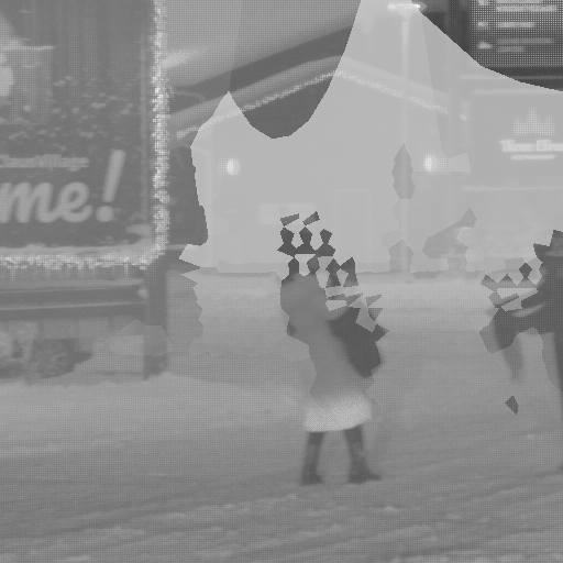
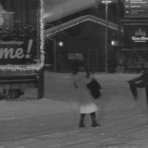
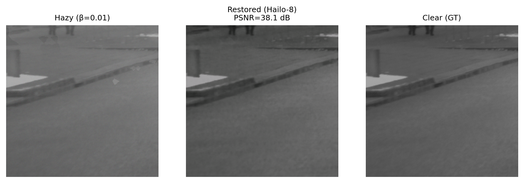
Real STF fog frames have no ground truth, so we measure agreement between the direct and physics heads. Agreement is higher in dense fog, where the gradient amplification concentrates learning.

**Table 5.** Dual-head consistency on real STF fog.
Metric	Dense fog	Light fog
MSE ↓	0.0002	0.0006
PSNR (dB) ↑	37.48	33.83
Pearson r ↑	0.9947	0.9912

Extended Analysis

Additional experiments run during the review period, all with the publicly released checkpoints.

Proposition 1 holds on real data

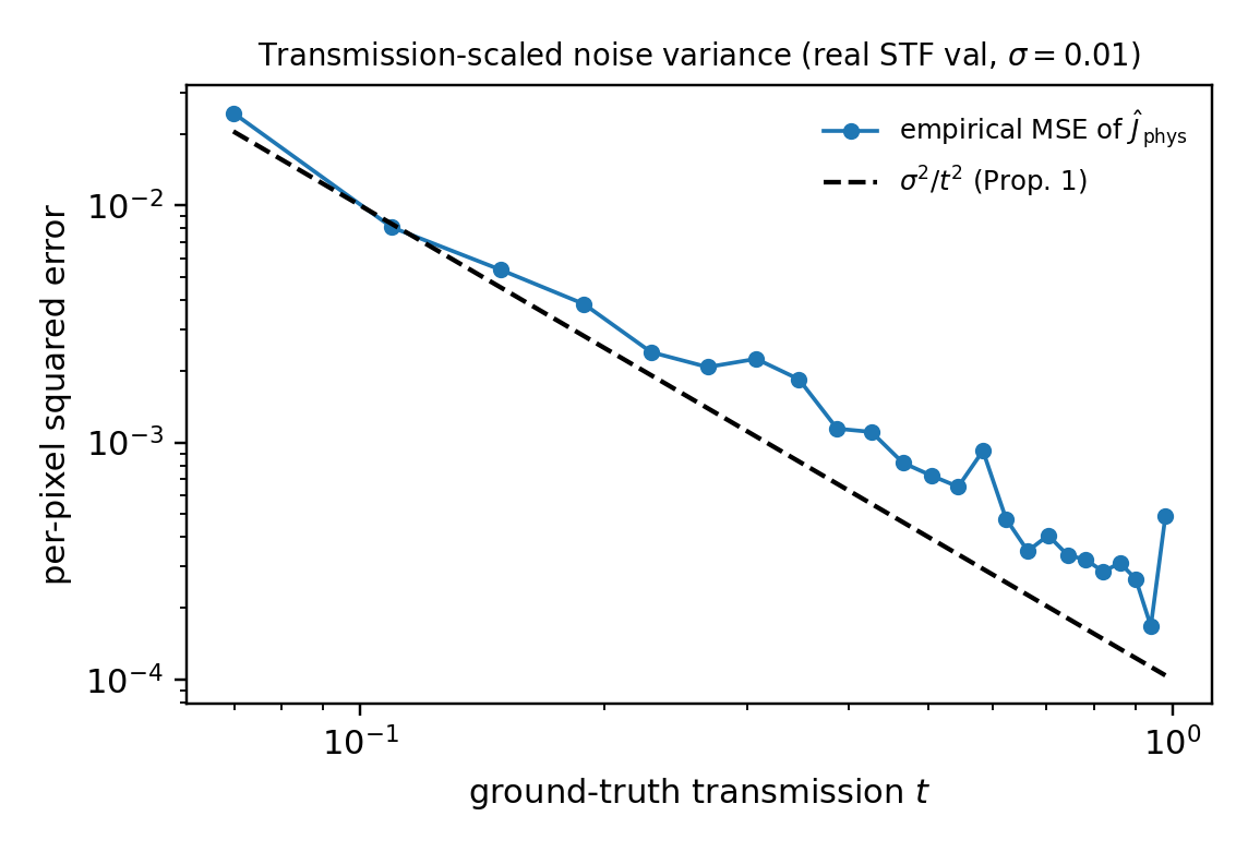
Log-log plot of per-pixel squared error of the physics inversion versus ground-truth transmission, following sigma squared over t squared — **Variance correspondence.** Per-pixel squared error of Ĵ_phys binned by ground-truth transmission on STF validation data (known noise σ = 0.01), against the σ²/t² law predicted by Proposition 1.

Proposition 1 predicts that the inversion's noise variance scales as Var[Ĵ_phys] = σ²/t² + O(δ), the same t⁻² structure that drives the gradient amplification. The measured error follows this law across two orders of magnitude, with a log-log correlation of r = 0.981. The small uniform offset above the line matches the O(δ) estimation term.

This also explains the noise visible in the physics head at low transmission (Fig. 11). It is the predicted variance structure, and the deployed direct head does not inherit it.

When does gradient amplification help?

We ran matched no-physics (NoPhy) controls on two further inverse problems and on RGB-only data. The mechanism helps when the inverted physical parameter is anchored by a privileged measurement such as depth. Without an anchor it is neutral, and it never hurts.

**Mechanism scope.** Physics variant vs. matched NoPhy twin, same architecture and budget.
Task	Inverted model	Anchored?	Physics vs. NoPhy
Dehazing, STF (NIR + sparse LiDAR)	t = e^−βd	yes, LiDAR	+5.51 dB PSNR, +0.99 pp mAP
Underwater restoration (NYU-v2 RGBD synth.)	per-channel t_c = e^−β_cd	yes, sparse depth	+0.38 dB overall, +0.82 dB mid-t bin, +0.60 dB red channel
Low-light, LOL-v2-Real (100 images)	Retinex R = I / (L + ε)	yes	+0.5 to 0.6 dB, SSIM 0.906 vs 0.897
Dehazing, RESIDE-6K (RGB only)	t = e^−βd	no	tie, 28.4 vs 28.6 dB
Low-light, LOL-v1 (15 images)	Retinex	no	inconclusive, noise-dominated test set

Low-light enhancement is the A → 0 special case of Eq. 5.

Robust to missing LiDAR and to RGB-only input

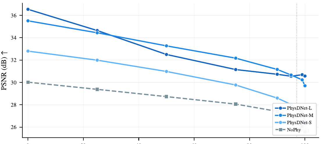
PSNR versus percentage of LiDAR points dropped for PhysDNet S, M, L and NoPhy — **Figure 9. PSNR vs. LiDAR dropout.** All variants degrade gracefully as LiDAR points are removed. At 0% density (NIR only) PhysDNet-M keeps 29.70 dB, still **+4.10 dB** above NoPhy. The dotted line marks the training-time density (~3% of pixels).

RGB-only training. PhysDNet-M trained from scratch on RESIDE-6K with zero depth input reaches 28.4 dB / 0.965 SSIM on the full 1,000-image SOTS-mix test set with the same recipe, and was still converging at the 300-epoch budget. It keeps the NPU-compatible operator set.

Depth branch folds away. With zero depth input the LiDAR branch's activations become constants that fold into the network. The outputs are bit-exact and compute drops from 8.56 to 6.33 GMACs (−26%) for RGB-only deployment.

The training regime drives transfer. Zero-shot on O-HAZE, the STF-trained model beats its colour-native RESIDE-trained sibling by about 3 dB PSNR-RGB (19.65 vs 16.58).

All weather conditions, day and night

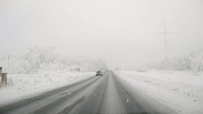
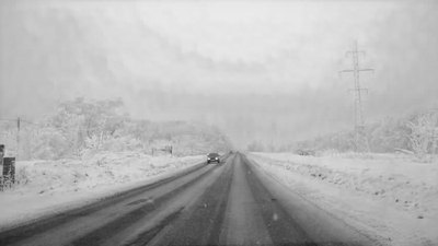
Dual-head consistency on real STF captures (real camera, real weather-attenuated LiDAR, n = 250 per split, full resolution) across every official split, including rain and snow, which were not in the paper.

**Weather robustness.** Direct ↔ physics head agreement, PSNR (dB) / Pearson r.
Condition	Day	Night
Clear	39.2 / 0.998	33.4 / 0.993
Light fog	40.1 / 0.999	34.7 / 0.994
Dense fog	40.3 / 0.999	34.8 / 0.995
Snow	39.5 / 0.997	35.4 / 0.994
Rain	35.1 / 0.995	—

Agreement is highest in dense fog, as the density-adaptive mechanism predicts. Night scenes lose a uniform ~5 dB with r ≥ 0.993, because active light sources locally violate the global-airlight assumption; the direct head absorbs this.

Dense fog, day: input, direct head, physics inversion — Dense fog, day

Light fog, night: input, direct head, physics inversion — Light fog, night

Snow, night: input, direct head, physics inversion — Snow, night

Rain: input, direct head, physics inversion — Rain

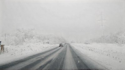
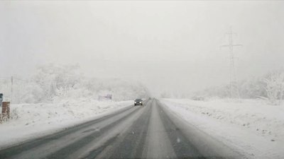
Each strip: real input, direct head, physics inversion.

Real-world haze without labels (RTTS)

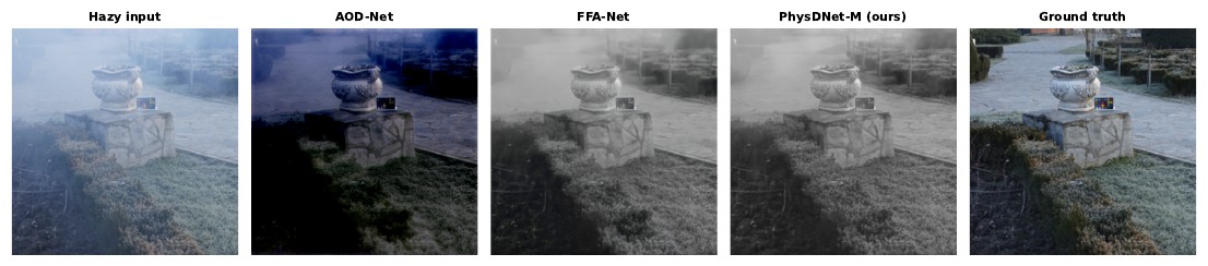
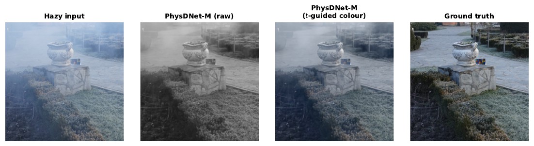
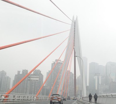
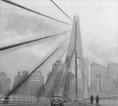
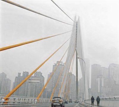
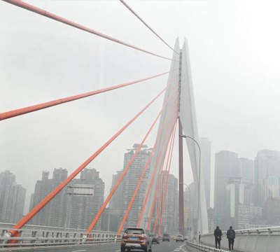
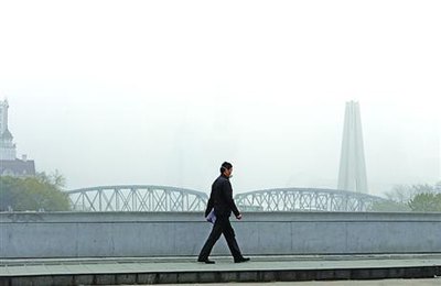
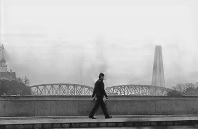
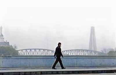
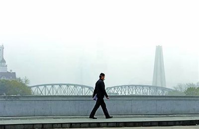
Trained on monochrome NIR, PhysDNet's raw output on RGB haze is nearly grey. We replace the paper's heuristic colour transfer with label-free self-supervised adaptation on unpaired real haze. The parameter-free physics inversion acts as a colour teacher: it is closed-form algebra on the coloured input, so its output is inherently coloured. The recipe adds Koschmieder re-composition, dual-head consistency, a dark-channel prior and synthetic replay, needs no architecture change, and takes 5 epochs (about 13 minutes on one 16 GB GPU).

Hazy input

Zero-shot (STF)

+ URHI adaptation

+ RTTS adaptation, physics head

**RTTS** (1,297 real hazy images, full resolution). Detection: YOLOv8-M mAP@0.5 against RTTS boxes.
Condition	Colorfulness	NIQE ↓	BRISQUE ↓	mAP@0.5
Hazy (unprocessed)	15.70	5.35	38.3	48.14
PhysDNet-M, zero-shot STF	0.03	4.90	34.7	46.28
+ URHI adaptation (unpaired, no labels)	12.83	4.74	33.4	44.82
+ RTTS-train adaptation, physics head	16.49	5.11	36.5	48.21
PhysDNet-M, RESIDE-6K-trained	19.45	4.81	33.6	47.71

URHI adaptation restores colour (0.03 → 12.8) and gives the best no-reference quality of all conditions. Adapted on RTTS's own unlabeled train split, the physics head matches or exceeds the raw hazy input on every measured axis. We report the trade-offs too. RTTS haze is mostly light and COCO-pretrained YOLO is already haze-robust, so direct-head outputs lower mAP there. The URHI-adapted model also gives up 5.1 dB on O-HAZE's dense machine haze, so Table 4 keeps the base model. Colour fidelity inherits the airlight estimate, so a mild warm shift can appear under strongly tinted light.

Edge Deployment

PhysDNet uses only NPU-friendly operators (depthwise-separable convolutions, BatchNorm, ReLU6, bilinear upsampling). Under standard ONNX export and vendor INT8 post-training quantization, only PhysDNet and AOD-Net compile for the fixed-function NPU, and AOD-Net's restoration quality (20.95 dB) is insufficient for deployment.

**Table 6.** 256×256, batch 1. Fixed-function 26 TOPS NPU (<4 W TDP) uses INT8 PTQ; Jetson Orin Nano uses TensorRT FP16. ✗ = compilation failure.
			Fixed-function NPU		Jetson Orin Nano
Model	Params (M)	GMACs	Compile	FPS	FPS	Power (W)
AOD-Net LiDAR	0.002	0.06	✓	1220	327.0	4.94
FFA-Net LiDAR	0.77	24.68	✗	—	46.9	8.21
DehazeFormer-T LiDAR	1.36	2.73	✗	—	47.1	12.38
DEA-Net LiDAR	3.65	16.44	✗	—	28.5	10.17
PhysDNet-S	0.72	2.24	✓	99	108.3	13.45
PhysDNet-M	2.95	8.56	✓	45	58.5	12.38
PhysDNet-L	6.59	18.98	✓	29	38.8	11.80

Recent heavyweight and diffusion methods, measured

The paper excludes 2024–2026 heavyweight and diffusion dehazers as outside the edge budget. We measured them under the same protocol: fvcore at 256², Jetson Orin Nano in MAXN (25 W) mode, TensorRT FP16, 50 warm-up + 300 timed iterations, engine build excluded.

**Excluded methods on Jetson Orin Nano.** NFE = network evaluations per image.
Method	Params	GMACs / call	NFE	Effective GMACs	Jetson, TRT FP16
UVM-Net (official)	1004 M	250.9	1	250.9	fails (out of memory)
DFFNet^‡	17.8 M	61.3	1	61.3	no ONNX (2-D FFT); 157 ms eager
Ksformer^‡	5.5 M	109.0	1	109.0	360 ms (2.8 FPS)
DehazeDDPM (official)	97.8 M	90.2	50	4509	3.1 s / image (0.32 FPS)
RSHazeDiff (official)	109.7 M	8.0	1690	13523	17.0 s / image (0.06 FPS)
PhysDNet-L	6.59 M	18.98	1	18.98	25.8 ms (38.8 FPS)

^‡Faithful re-implementations calibrated to the published parameter budgets; no official code exists. Even PhysDNet-L needs 3.2× less compute than the lightest excluded method, and those methods' INT8 behaviour, required at NPU power budgets, is uncharacterised.

Hazy input, NPU output at 38.1 dB, ground truth — **Figure 5. INT8 NPU inference on a representative STF sample (β = 0.01).** Hazy input, PhysDNet-M restored on the fixed-function NPU (38.1 dB), and ground truth.

BibTeX

@inproceedings{dhahri2026physdnet,
  title     = {PhysDNet: Physics-Driven Gradient Amplification for
               Real-Time Image Dehazing},
  author    = {Dhahri, Rayen and Sun, Lei and Kartsch Morinigo, Victor Javier
               and Pagnoux, Alice and Benini, Luca and Paudel, Danda Pani
               and Van Gool, Luc},
  booktitle = {Advances in Neural Information Processing Systems (NeurIPS)},
  year      = {2026}
}